LAB 1. TFP Distributions

LAB 1. TFP Distributions#

import inspect
from rlxmoocapi import submit, session

import numpy as np
import matplotlib.pyplot as plt
import seaborn as sns
import tensorflow as tf
import tensorflow_probability as tfp
from scipy import stats

tfd = tfp.distributions
tfb = tfp.bijectors

course_id = "ppdl.v1"
endpoint = "https://m5knaekxo6.execute-api.us-west-2.amazonaws.com/dev-v0001/rlxmooc"
lab = "L02.03.01"

session.LoginSequence(
    endpoint=endpoint,
    course_id=course_id,
    lab_id=lab,
    varname="student"
    );

Task 1#

Manually compute the pdf for different batch and event shapes, without using tensorflow_probability. You must use numpy and scipy.stats to replicate the following distribution:

def tf_random_normal_pdf(x, mu, cov):
    dist = tfd.MultivariateNormalTriL(
            loc=mu, scale_tril=tf.linalg.cholesky(cov)
            )
    return dist.log_prob(x)

sample_size = 5
batch_size = 3
event_size = 2

mu = (
        np.random.uniform(
            0, 1, size=(batch_size, event_size)
            )
        .astype(np.float32)
        )
cov = (
        np.random.uniform(
            1, 2, size=(event_size, event_size)
            )
        .astype(np.float32)
        )
cov = cov.dot(cov.T) # Ensuring PSD matrix

x = (
        np.random.normal(
            loc=2, scale=5,
            size=(sample_size, batch_size, event_size)
            )
        .astype(np.float32)
        )
tf_random_normal_pdf(x, mu, cov)

We suggest using scipy.stats.multivariate_normal:

def random_normal_pdf(x, mu, cov):
    ...

random_normal_pdf(x, mu, cov)

Test your code:

student.submit_task(namespace=globals(), task_id="T1");

Task 2#

The probability for a person to default on a credit depends on his income, and it is modeled with a distribution depending on the person’s age \(x_i\), older people have flatter exponentials, meaning that as you get older the probability of default for higher incomes is higher than we you are younger.

Observe how we want to assign a distribution to each data point

Make a function that, given a set of \(x\in\mathbb{R}^n\), returns a batched distribution of batch_size\(=n\) that assigns to each \(x_i\) a \(\mathcal{N}(\mu_i, \sigma_i)\) so that:

\(\mu_i = 2 x_i\).
\(\sigma_i = \text{softplus}(x_i, \beta=\frac{1}{5}) = 5 \text{log}(\text{exp}(5 x) + 1)\)

def credit_exp_dist(x):
    ...

x = np.linspace(18, 60, 100)
dist = credit_exp_dist(x)

Run the next cell to visualize the scoring distribution for the learned distribution, it must look similar to the following image:

credit exponential distribution

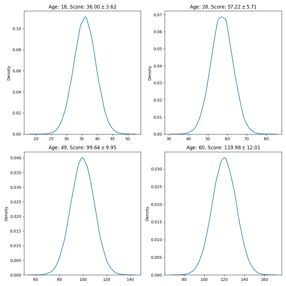
customers = [0, 25, 75, 99]
fig, ax = plt.subplots(2, 2, figsize=(10, 10))
sample = dist.sample(100000).numpy()
for i, customer in enumerate(customers):
    axi = ax[i // 2, i % 2]
    sns.kdeplot(sample[:, customer], ax=axi);
    axi.set_title(f"Age: {int(x[customer])}, Score: ${sample[:, customer].mean():.2f}\\pm {sample[:, customer].std():.2f}$")
fig.tight_layout()

Test your code:

student.submit_task(namespace=globals(), task_id="T2");

Task 3#

Now, We want to implement a multivariate batch distribution, such that each data point is described by more variables, not only the person’s age. In this case, We’ll be using the age and the years of laboral experience of a given customer, you must implement:

\(y_{i, 0} \sim \mathcal{N}(\mu_{i, 0}, \sigma_{i, 0})\).
\(y_{i, 1} \sim \mathcal{N}(\mu_{i, 1}, \sigma_{i, 1})\).
\(\text{score_i} = y_{i, 0} + y_{i, 1}\).
\(\mu_{i, 0} = 2 x_i\).
\(\mu_{i, 1} = -x_i\).
\(\sigma_{i, 0} = \text{softplus}(x_i, \beta=\frac{1}{5})\).
\(\sigma_{i, 1} = \text{softplus}(x_i, \beta=\frac{1}{2})\).

Where \(y_{i, 0}\) is the credit score assigned to the age and \(y_{i, 1}\) is the credit score assigned to the years of experience for the \(i\)-th customer.

def credit_mult_dist(x):
    ...

age = np.linspace(18, 60, 100)
experience = np.array([np.random.randint(0, i) for i in age])
X = np.vstack([age, experience]).T

dist = credit_mult_dist(X)
print(dist)

customers = [0, 25, 75, 99]
sample = dist.sample(10_000).numpy()
print(sample.shape)

Use the following cell to visualize the age distribution, the figure must look similar to this one:

Credit score and age

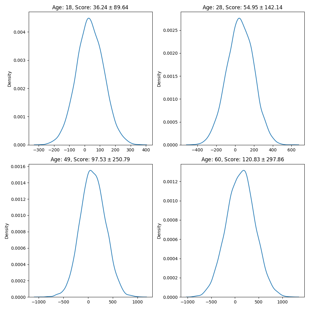
fig, ax = plt.subplots(2, 2, figsize=(10, 10))
for i, customer in enumerate(customers):
    sample_age = sample[..., 0]
    axi = ax[i // 2, i % 2]
    sns.kdeplot(sample_age[:, customer], ax=axi);
    axi.set_title(f"Age: {int(X[customer, 0])}, Score: ${sample_age[:, customer].mean():.2f}\\pm {sample_age[:, customer].std():.2f}$")
fig.tight_layout()

Use the following cell to visualize the years of experience distribution, the figure must look similar to this one:

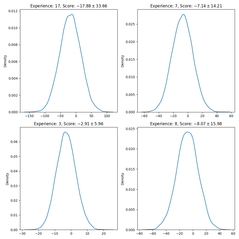Credit and years of experience Credit score distribution on years of experience

fig, ax = plt.subplots(2, 2, figsize=(10, 10))
for i, customer in enumerate(customers):
    sample_exp = sample[..., 1]
    axi = ax[i // 2, i % 2]
    sns.kdeplot(sample_exp[:, customer], ax=axi);
    axi.set_title(f"Experience: {int(X[customer, 1])}, Score: ${sample_exp[:, customer].mean():.2f}\\pm {sample_exp[:, customer].std():.2f}$")
fig.tight_layout()

Use the following cell to visualize the overall score distribution, the figure must look similar to this one:

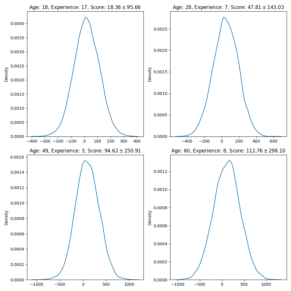
Overall credit score distribution

fig, ax = plt.subplots(2, 2, figsize=(10, 10))
for i, customer in enumerate(customers):
    sample_overall = sample.sum(axis=-1)
    axi = ax[i // 2, i % 2]
    sns.kdeplot(sample_overall[:, customer], ax=axi);
    axi.set_title(f"Age: {int(X[customer, 0])}, Experience: {int(X[customer, 1])}, Score: ${sample_overall[:, customer].mean():.2f}\\pm {sample_overall[:, customer].std():.2f}$")
fig.tight_layout()

student.submit_task(namespace=globals(), task_id="T3");

Task 4#

In this task, you must implement the tfb.Scale bijector using scipy and numpy without tensorflow.

Suppose We have the following distribution for a random variable \(x\).

\[ x \sim \mathcal{Beta}(a, b) \]

And that we want to compute the logpdf of the following random variable:

\[ y = f(x) = k \cdot x \]

The PDF for y would be:

\[\begin{split} \text{log}(P_y(x)) = \text{log}(P_x(f^{-1}(x))) + \log \text{det}\Big[\frac{\partial}{\partial x} f^{-1}(x) \Big] \\ \end{split}\]

And in this case, since \(x\) is a scalar (single variable distribution):

\[\begin{split} \begin{align} f^{-1}(x) &= \frac{x}{k}\\ \text{det}\Big[\frac{\partial}{\partial x} f^{-1}(x) \Big] &= \frac{\partial}{\partial x} f^{-1}(x) = \frac{1}{k} \end{align} \end{split}\]

Finally:

\[ \text{log}(P_y(y)) = \text{log}(P_x(\frac{x}{k})) + \text{log}(\frac{1}{k}) \]

# distribution parameters
a = np.random.uniform(0.1, 3)
b = np.random.uniform(0.1, 3)
k = np.random.uniform(1, 10)

Take a look at the expected bijector:

dist = tfb.Scale(k)(tfd.Beta(a, b))

def scale_beta_logpdf(x, a, b, k):
    ...

The following subplots must look the same:

x = np.linspace(0, 1, 100)
fig, ax = plt.subplots(1, 2, figsize=(10, 7))
ax[0].plot(x, np.log(dist.prob(x)))
ax[1].plot(x, scale_beta_logpdf(x, a, b, k))

student.submit_task(namespace=globals(), task_id="T4");